
Running one-sample t-test in SPSS statistics
Analysis of one sample t-test in SPSS
The test is used to determine whether the sample data comes from a population with a specified mean. The one-sample t-test applies to situations where the population standard deviation is not known, although it is expected that the distribution of the data should be approximately normal. This population mean is always hypothesized as it is always not known. Before conducting data analysis using any statistical procedure, it is important to know the assumptions that are associated with the test. The assumptions that must be met by your data before conducting your analysis using a one-sample t-test are as follows.
Assumptions for a one-sample t-test
Assumption 1: The outcome variable should be measured at the ratio or the interval ratio. That is, the variable should be on a continuous scale.
Assumption 2: Each observation should be independent of any other observation. i.e independence of the data.
Assumption 3: There should be no significant outliers in your data.
Assumption 4: The distribution of your observations should be approximately normal.
Example and setup of one-sample data in SPSS
For a one-sample t-test, there will only be one variable, to be entered into the software.
In this case, we would wish to test whether the average depression scores of the sampled students is equal to the national average of 4.0. To do this we recruit 40 participants to take part in the study. The data has been entered in SPSS.
One-sample t-test step by step analysis in SPSS
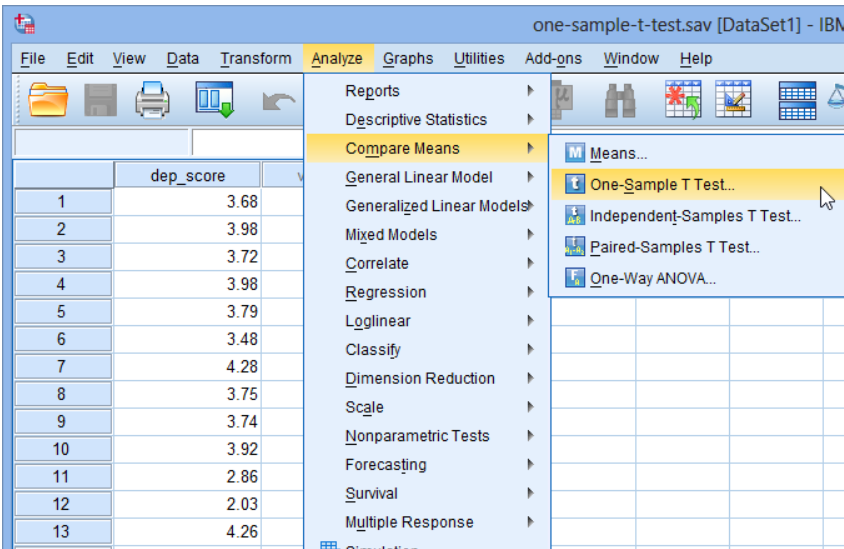
Step 1: Click Analyze > Compare Means > One-Sample T-Test as shown in the screenshot below.
The variable for the depression score has been recorded.
Step 2: In the one-sample t-test dialogue box presented, transfer the variable to the test variable box, and enter the population value you are comparing with the sample data to the Test value box. as shown in the image below.
Step 3: Click on options in you would wish to construct a 95% confidence interval and enter 95% in the box.
Last step: Click continue and click okay to get your output.
The output, including the descriptive analysis, will be as shown below.
you can make an initial interpretation of the data using the One-Sample Statistics table, which presents relevant descriptive statistics:
It is more common than not to present your descriptive statistics using the mean and standard deviation ("Std. Deviation" column) rather than the standard error of the mean ("Std. Error Mean" column), although both are acceptable. You could report the results, using the standard deviation, as follows:
Mean depression score (3.72 ± 0.74) was lower than the population 'normal' depression score of 4.0.
One-sample t-test table
Note that, the p-value indicates the probability of obtaining the observed t-value if the null hypothesis is correct.
Reporting your results.
Depression score was statistically significantly lower by a mean of 0.26, 95% CI [0.04 to 0.51], than a normal depression score of 4.0, t(39) = -2.381, p = .022.


Comments (0)