
Binomial logistic regression using SPSS IBM statistics
Binomial logistic is simply a logistic regression model that can be used to predict the probability of an outcome falling within a given category. The dependent variable is always a dichotomous variable and the predictors (independent variables) can be either continuous or categorical variables. When there are more than two categories of the outcome variables, then it is appropriate to use a multinomial logistic regression model. An example is when one might be interested in predicting whether a student "passes" or "fails" his/her college statistics based on the time they spend while revising for the exam. One can also predict the probability of drug use based on previous behaviors, age, and gender.
This text explains to you the best way to do binomial regression using SPSS Statistics. However, before we run the data through a binomial process, your data must meet the following assumptions.
Assumptions for a Binomial regression model
1. The dependent variable should be on a dichotomous scale - That is the measurements of the variables should be measured in categorical form. Examples of categorical variables include gender, race, presence of heart disease (Yes or No). Remember that we also have an ordinal regression model which can be used when the response variable is on an ordered scale.
2. You must have more than one independent variable measured on either a continuous scale, an ordered scale or a categorical scale.
3. The independence of the observations should also be met.
4. Your continuous variable and the logit transformation of the dependent variable must be linearly related.
The 4th assumption can be checked via SPSS but the first three assumptions relate to the data collection process,
Case:
In this example, we analyze to predict heart-disease (The dependent variable), that is whether an individual has heart disease or no, Using maximal aerobic capacity, age, weight, and gender. Note that age and weight are the continuous variables while gender is the categorical predictor variables.
Analysis:
To run the Logistic regression model in SPSS step by step solutions
Step 1: Go to Analyze > Regression > Binary Logistic as shown in the screenshot below.
Step 2: In the logistic regression dialogue box that appears, transfer your dependent variable to the dependent variable (in this case its heart_disease) dialogue box and move you independent variables to the covariate dialogue box.
The dialogue box shows how the variables should be transferred.
Step 3: Click categorical to define the categorical variables (Gender), and transfer your categorical variables to the categorical covariates as shown below.
Step 4: See the contrast area check the first option in the contrast category and click the Change button as shown below.
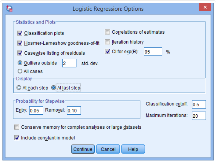
Step 5: Click continue to return to the logistic dialogue box the Options button the dialogue box below is presented.
Step 6: Check the following buttons, Classification plots, Hosmer-Lemeshow goodness of fit and casewise listing of residuals in the statistics and plots and the CI for Exp(b). Remember to check the at last step in the display area. Your dialogue box after this step should be as shown below.
Last step: Click continue to return to your logistic regression dialogue box and click OK to get your output.
Output and interpretation of the Logistic results
Variance Explained
This is equivalent to the R-squared explained in the multiple regression model. Cox & Snell R Square and Nagelkerke R Square values are used to explain the variation that can be explained by the model. Based on the output of the model, the explained variation is between 0.240 and 0.330 it is upon you to pick the statistic that interests you. Nagelkerke R2 is a modification of Cox & Snell R2, the latter of which cannot achieve a value of 1. Remember that it is always advisable to report the Nagelkerke statistics because Cox ^ Snell cannot be 1.
Classification table
The cut value of 0.50 implies that if the predicted category is greater than 0.50 then that is classified as a "Yes" otherwise that is a no.
Some useful information that the classification table provides include:
- A. The percentage accuracy in classification (PAC), which reflects the percentage of cases that can be correctly classified as "no" heart disease with the independent variables added (not just the overall model).
- B. Sensitivity, which is the percentage of cases that had the observed characteristic (e.g., "yes" for heart disease) which were correctly predicted by the model (i.e., true positives).
- C. Specificity, which is the percentage of cases that did not have the observed characteristic (e.g., "no" for heart disease) and were also correctly predicted as not having the observed characteristic (i.e., true negatives).
- D. The positive predictive value, which is the percentage of correctly predicted cases "with" the observed characteristic compared to the total number of cases predicted as having the characteristic.
- E. The negative predictive value, which is the percentage of correctly predicted cases "without" the observed characteristic compared to the total number of cases predicted as not having the characteristic.
Variables in the equation table
The table presents the contribution of each variable and its associated statistical significance.
The wald statistic determines the statistical significance of each independent variable. From these results it be seen that age (p = .003), gender (p = .021) and VO2max (p = .039) added significantly to the model, weight (p = .799) did not. You can use the information in the "Variables in the Equation" table to predict the probability of an event occurring based on a one-unit change in an independent variable when all other independent variables are kept constant. For example, the table shows that the odds of having heart disease ("yes" category) is 7.026 times greater for males as opposed to females.


Comments (0)